2.1 Ice-sheet model and simulations

We perform simulations of the response of the Antarctic ice sheet (Fig. 1a) to environmental and parametric perturbations over the period 2000–3000 CE with the fast Elementary Thermomechanical Ice Sheet (f.ETISh) model (Pattyn, 2017) version 1.2. The f.ETISh model is a vertically integrated, thermomechanical, hybrid ice-sheet/ice-shelf model that incorporates essential characteristics of ice-sheet thermomechanics and ice-stream flow, such as the mass-balance feedback, bedrock deformation, sub-shelf melting and calving. The ice flow is represented as a combination of the shallow-ice (SIA) (Hutter, 1983; Greve and Blatter, 2009) and shallow-shelf (SSA) (Morland, 1987; MacAyeal, 1989; Weis et al., 1999) approximations for grounded ice (Bueler and Brown, 2009), while only the shallow-shelf approximation is applied for floating ice shelves. Bedrock deformation is represented as a combined time-lagged asthenospheric relaxation and elastic lithospheric response (Greve and Blatter, 2009; Pollard and DeConto, 2012a), in which the lithosphere relaxes towards isostatic equilibrium due to the viscous properties of the underlying asthenosphere. Calving at the ice front is parameterised based on the large-scale stress field, represented by the horizontal divergence of the ice-shelf velocity field (Pollard and DeConto, 2012a). Prescribed input data include the present-day ice-sheet geometry and bedrock topography from the Bedmap2 dataset (Fretwell et al., 2013), the basal sliding coefficient, and the geothermal heat flux by An et al. (2015).

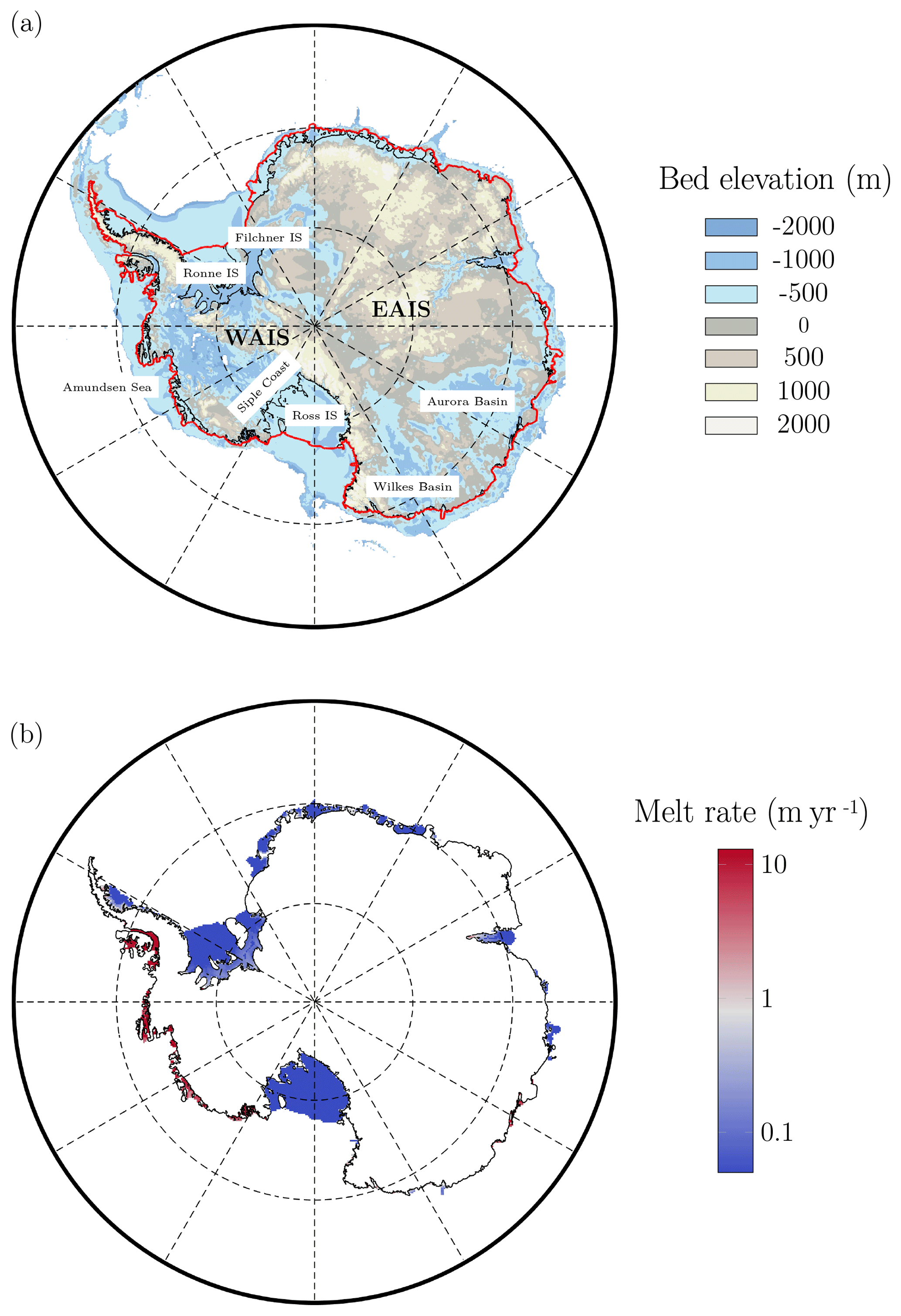
Figure 1Antarctic bedrock topography and sub-shelf melting. (a) Bedrock topography (m a.s.l.) (Fretwell et al., 2013) of the present-day Antarctic ice sheet and geographic features. WAIS is the West Antarctic ice sheet, EAIS is the East Antarctic ice sheet and IS is ice shelf. Grounding line is shown in black and ice front is shown in red. (b) Sub-shelf melt rate for the present-day Antarctic ice sheet computed with the PICO ocean model (Reese et al., 2018a). Refreezing under ice shelves is not allowed.

Download

We perform simulations at a spatial resolution of 20 km while accounting for grounding-line migration at coarse resolution with a flux condition derived from a boundary layer theory at steady state based on either a Weertman (or power) friction law (Schoof, 2007b) or a Coulomb friction law (Tsai et al., 2015) at the grounding line. This flux condition at the grounding line is imposed as an internal boundary condition following the implementation by Pollard and DeConto (2009, 2012a). This implementation has been shown to reproduce the migration of the grounding line and its steady-state behaviour (Schoof, 2007a) at coarse resolution for the SSA and hybrid SSA/SIA models, while these models can only reproduce the migration of the grounding line and its steady-state behaviour at sufficiently fine resolution in the absence of a flux condition (Docquier et al., 2011; Pattyn et al., 2012). Numerical simulations (Pollard and DeConto, 2012a; DeConto and Pollard, 2016) of the Antarctic ice sheet using a flux condition have also been able to reproduce MISI in large-scale ice-sheet simulations. In addition, Pattyn (2017) has shown that a flux condition makes the f.ETISh model rather independent of the resolution for a spatial resolution of the order of 20 km. While the implementation of a flux condition at the grounding line has been shown to reproduce qualitatively ice-sheet dynamics as determined with other ice-sheet models, it cannot reproduce quantitatively changes in ice-sheet mass and the contribution to sea level as determined from models with a higher level of complexity, such as the Blatter–Pattyn (Blatter, 1995; Pattyn, 2003) and full Stokes (Greve and Blatter, 2009) models that include vertical shearing at the grounding line, especially for short transients (decadal timescales) as these flux conditions have been derived at steady state (Drouet et al., 2013; Pattyn et al., 2013; Pattyn and Durand, 2013). A proper representation of grounding-line migration without the need for a flux condition would require a very fine grid resolution (possibly less than 200 m). In addition, the flux condition has been derived for unbuttressed ice shelves (Schoof, 2007b) and may fail to appropriately represent grounding-line migration for buttressed ice shelves (Reese et al., 2018b) as found mostly around Antarctica even when the flux condition is corrected for buttressing with a buttressing factor accounting for back stress at the grounding line. In particular, Pattyn et al. (2013) have shown that models that implement the flux condition cannot reproduce compressional stresses that may apply in the presence of buttressing. Moreover, using a spatial resolution of 20 km does not allow us to capture properly certain mechanisms that control grounding-line migration such as bedrock irregularities and ice-shelf pinning points even with sub-grid parameterisations of these mechanisms. Therefore, we may expect discrepancies between our results and results at higher spatial resolutions (<5 km), especially for important small ice streams such as Pine Island and Thwaites glaciers, which represent only a few grid points with a 20 km resolution. Despite the limitations of the flux condition and our coarse grid resolution, we have adopted these modelling assumptions as an efficient way to capture the essential mechanisms of grounding-line migration in large-scale, long-term and large-ensemble ice-sheet simulations while keeping the computational cost tractable. The computational cost of a single forward simulation with a time step of 0.05 years on the CÉCI clusters (F.R.S-FNRS & Walloon Region) on two threads is approximately 8 h. To investigate the impact of the spatial resolution on the results, we performed additional runs at a spatial resolution of 16 km (Fig. S1 in the Supplement). We found that the uncertainty in the projections due to the spatial resolution is (far) less important than the uncertainty due to the uncertainty in the parameters.

The main changes in f.ETISh version 1.2 as compared to version 1.0 (Pattyn, 2017) consist of the computation of sub-shelf melt rates with an ocean-model coupler based on the Potsdam Ice-shelf Cavity mOdel (PICO) ocean-model coupler (Reese et al., 2018a) rather than simpler parameterisations of sub-shelf melt rates (Beckmann and Goosse, 2003; Holland et al., 2008; Pollard and DeConto, 2012a; de Boer et al., 2015; Cornford et al., 2016), the inclusion of a laterally varying flexural rigidity for the lithosphere (Chen et al., 2018) to compute glacial isostatic adjustment more realistically with an elastic lithosphere/relaxed asthenosphere model, an improvement of the SSA numerical scheme based on the implementation by Rommelaere and Ritz (1996) and a description of atmospheric forcing based on a parameterisation of the changes in atmospheric temperature and precipitation rate (Huybrechts et al., 1998; Pollard and DeConto, 2012a), a parameterisation of surface melt with a positive degree-day model (Janssens and Huybrechts, 2000) and the inclusion of meltwater percolation and refreezing (Huybrechts and de Wolde, 1999).

We drive our simulations with both atmospheric and oceanic forcings. Present-day mean surface air temperature and precipitation are obtained from Van Wessem et al. (2014), based on the regional atmospheric climate model RACMO2. Changes in atmospheric temperature and precipitation rate induced by a forcing temperature change ΔT are applied in a parameterised way that accounts for elevation changes (Huybrechts et al., 1998; Pattyn, 2017). We use a positive degree-day (PDD) model to calculate surface melt (Janssens and Huybrechts, 2000), assuming a PDD factor of 3 and 8 mm ^∘C⁻¹ d⁻¹ for snow and ice, respectively. The PDD model also includes meltwater percolation and refreezing (Huybrechts and de Wolde, 1999).

Basal melting underneath ice shelves is determined from the PICO ocean-model coupler (Reese et al., 2018a), which evaluates sub-shelf melting from the ocean temperature T_oc and salinity fields on the continental shelf via an ocean box model that captures the basic overturning circulation within ice-shelf cavities. We employ data by Schmidtko et al. (2014) for present-day ocean temperature $T_{\mathrm{oc}}^{\mathrm{obs}}$ and salinity on the continental shelf. For a change in background atmospheric temperature ΔT, we assume that the ocean temperature T_oc on the continental shelf changes as

where F_melt is an ocean melt factor that represents the ratio between oceanic and atmospheric temperature changes (Maris et al., 2014; Golledge et al., 2015). Equation (1) with F_melt=0.25 has been shown to reproduce trends in ocean temperatures following an analysis of the Climate Model Intercomparison Project phase 5 (CMIP5) data set (Taylor et al., 2012) for changes in atmospheric and ocean temperatures (Golledge et al., 2015). Figure 1b shows the initial sub-shelf melt rate as computed with the PICO model. The PICO model is able to reproduce the general pattern of sub-shelf melting with higher melt rates near the grounding line and lower melt rates near the calving front. Sub-shelf melt rates are also higher in the Amundsen Sea sector and lower underneath the large Ross and Filchner–Ronne ice shelves.

The calibration of the basal sliding coefficient follows the data assimilation method of ice-sheet geometry by Pollard and DeConto (2012b). This approach is based on a fixed-point iteration scheme that adjusts the basal sliding coefficient iteratively so as to match the present-day ice-sheet configuration while assuming that the present-day configuration is in steady state. After applying this approach, we further adjust the basal sliding coefficient in ice streams with a sliding multiplier factor similar to Bindschadler et al. (2013) to reduce the initial drift. We carry out the calibration step independently for the different sliding and grounding-line flux conditions investigated in this paper. For the nominal values of the model parameters and without forcing anomaly, the initial drifts (reference runs) range from 0.1 to 0.2 m of sea-level rise by 3000. To make our analysis insensitive to model initialisation, we correct all our results for this initial bias by subtracting the reference runs from the results. Therefore, after corrections for present-day dynamical changes, our results reflect the model response to perturbations. These corrections have in general little impact on medium-term and long-term projections as the initial drift is small compared to the projections but leads to a more significant bias for short-term projections.

2.2 Sources of uncertainty

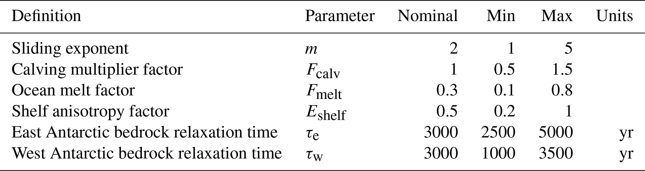
We aim at quantifying the response of the Antarctic ice sheet to climate change while accounting for uncertainty in atmospheric forcing, basal sliding, grounding-line flux parameterisation, calving, sub-shelf melting, ice-shelf rheology and bedrock relaxation. We account for uncertainty in these physical processes by introducing uncertainty in parameters in the f.ETISh model (see Table 1). Here, we choose the uncertainty ranges for the parameters sufficiently large so as to encompass extreme conditions. The effect of choosing narrower uncertainty ranges for the parameters is discussed in Sect. 3.6. We assume the parameters to take the same value everywhere over the whole Antarctic ice sheet. This approach is likely to be conservative as the parameters may vary at least regionally. We refer to Schlegel et al. (2018) for a discussion about uncertainty quantification based on a partitioning of the ice-sheet domain. In the remainder of this section, we list the uncertain parameters and briefly discuss their influence on the AIS response.

Table 1List of parameters and parameter ranges used in the uncertainty analysis.

Download Print Version | Download XLSX

2.2.1 Atmospheric forcing

Alongside oceanic forcing, atmospheric forcing is generally considered to be the primary driver of future changes in the AIS mass balance (Lenaerts et al., 2016; Pattyn et al., 2018). Simulating atmospheric forcing over several centuries with regional climate models is computationally prohibitive. In addition, the accuracy of the climate models is limited by uncertainties such as the possible trajectories of anthropogenic greenhouse gas emissions. Therefore, we adopt here the four schematic extended representative concentration pathway (RCP) scenarios RCP 2.6, RCP 4.5, RCP 6.0 and RCP 8.5 introduced by Golledge et al. (2015) for temperature changes ΔT in the atmosphere (Fig. 2) as a means of representing different atmospheric forcings relevant for policymakers.

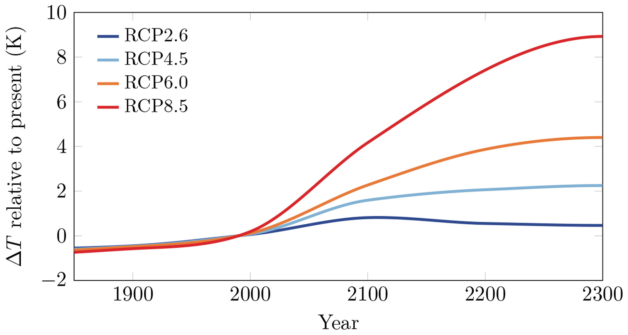
Figure 2Long-term RCP temperature scenarios (Golledge et al., 2015) for Antarctica (60–90^∘ S) based on the CMIP5 data (Taylor et al., 2012) and extended to 2300. Temperatures are held constant after 2300.

Download

The scenario plays a significant role in the amplitude and speed of the AIS retreat. Recent studies (Golledge et al., 2015; DeConto and Pollard, 2016) have shown no substantial retreat of the grounding-line position in the strongly mitigated RCP 2.6 scenario. The other scenarios lead to a reduction in the extent of the major ice shelves (Ross, Filchner–Ronne and Amery ice shelves) within 100–300 years, leading to accelerated grounding-line recession due to reduced buttressing. DeConto and Pollard (2016) have also highlighted that the hydrofracturing and ice-cliff failure mechanisms (not included in f.ETISh version 1.2) driven by increased surface melt and sub-shelf melting could potentially lead to an accelerated collapse of the West Antarctic ice sheet and a deeper grounding-line retreat in the East Antarctic subglacial marine basins.

2.3 Uncertainty quantification methods

3.1 Nominal projections

We first present nominal projections obtained using the nominal values of the parameters given in Table 1. We first present results under nominal conditions in order to assess subsequently the impact of uncertainties on AIS sea-level rise projections. Under nominal conditions, we find (Table 2) in RCP 2.6 an AIS contribution to sea level of 0.02 m by 2100, 0.07 m by 2300 and 0.20 m by 3000 and in RCP 8.5 an AIS contribution to sea level of 0.05 m by 2100, 0.59 m by 2300 and 3.90 m by 3000. In Fig. 3a, we represented the nominal projections as a function of time in all RCP scenarios. We find that the nominal AIS contribution to sea level is rather small in the first decades and starts to increase more significantly around 2100 with a rather constant growth rate. In Fig. 3b–e, we represented the nominal grounded ice region by 3000 for all RCP scenarios. We find that there is little ungrounding by 3000 in RCP 2.6 and RCP 4.5, while we observe a more significant ungrounding in Siple Coast and the Ronne basin in RCP 6.0 and a much more significant ungrounding in Siple Coast and the Amundsen Sea sector in RCP 8.5.

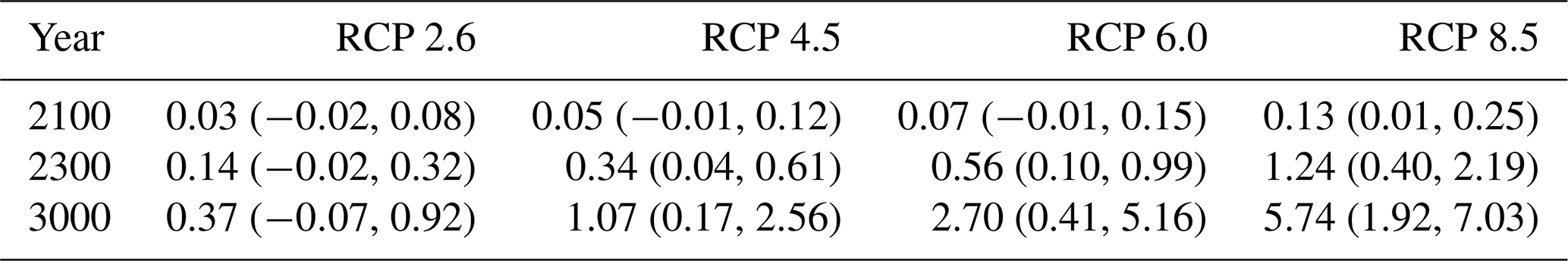
Table 2Nominal projections (in metres) of AIS contribution to sea level on short-term (2100), medium-term (2300) and long-term (3000) timescales in different RCP scenarios.

Download Print Version | Download XLSX

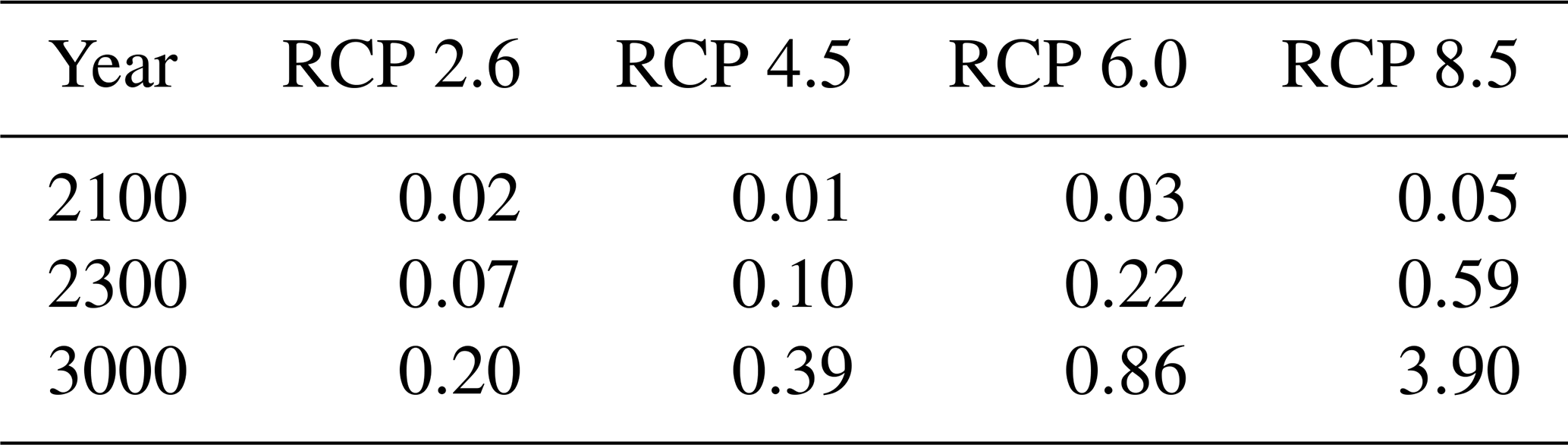
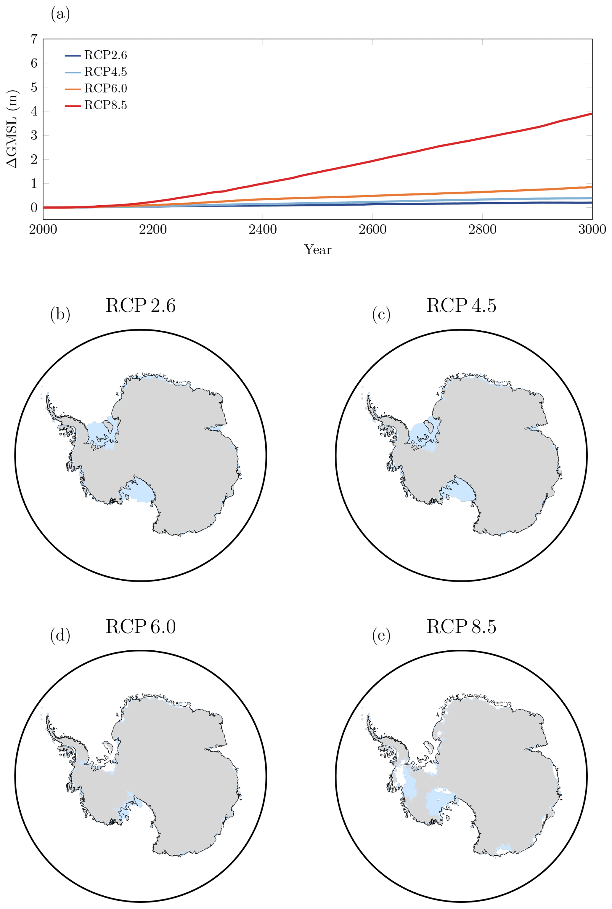
Figure 3(a) Nominal AIS contribution to sea level. Grounded ice (grey area) and ice shelves (light blue area) by 3000 in (b) RCP 2.6, (c) RCP 4.5, (d) RCP 6.0 and (e) RCP 8.5 for the nominal values of the parameters. The present-day grounding line is shown in black.

Download

3.2 Parameters-to-projection relationship

One of the advantages of a polynomial chaos expansion is that it provides an explicit approximation to the parameters-to-projection relationship, which can be visualised to gain insight into the relationship between the parameters and the projections.

In Figs. 4 and 5, we used the PC expansions to visualise how the projections depend on each parameter individually (one-at-a-time) while keeping the other parameters fixed at their nominal value under the weakly non-linear sliding law in RCP 2.6 and RCP 8.5, respectively.

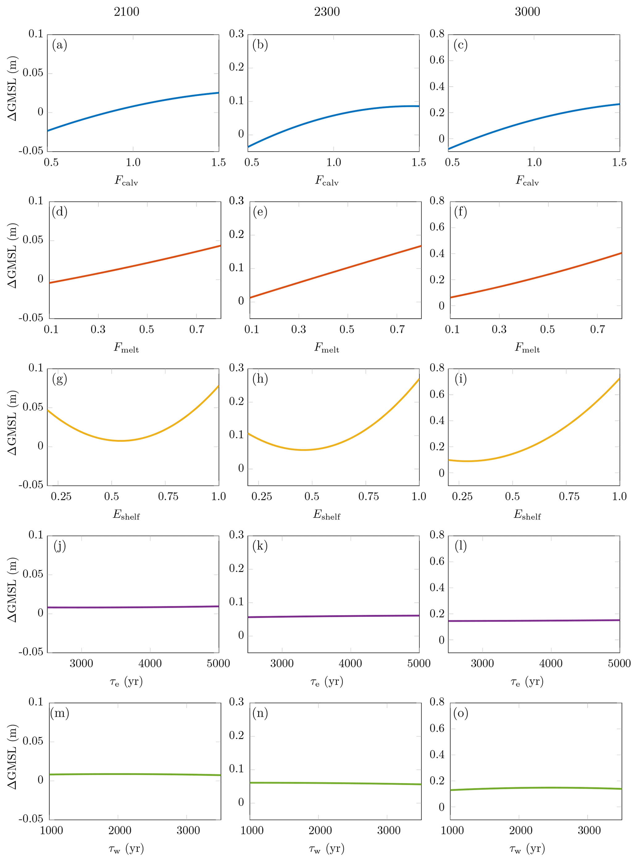
Figure 4Representation of the parameters-to-projection relationships in RCP 2.6 under the weakly non-linear sliding law as given by a PC expansion. The PC expansion is shown for each parameter individually, with the other parameters fixed at their nominal value. PC expansions at (a, d, g, j, m) 2100, (b, e, h, k, n) 2300 and (c, f, i, l, o) 3000.

Download

Figure 5Same as Fig. 4 but in RCP 8.5.

Download

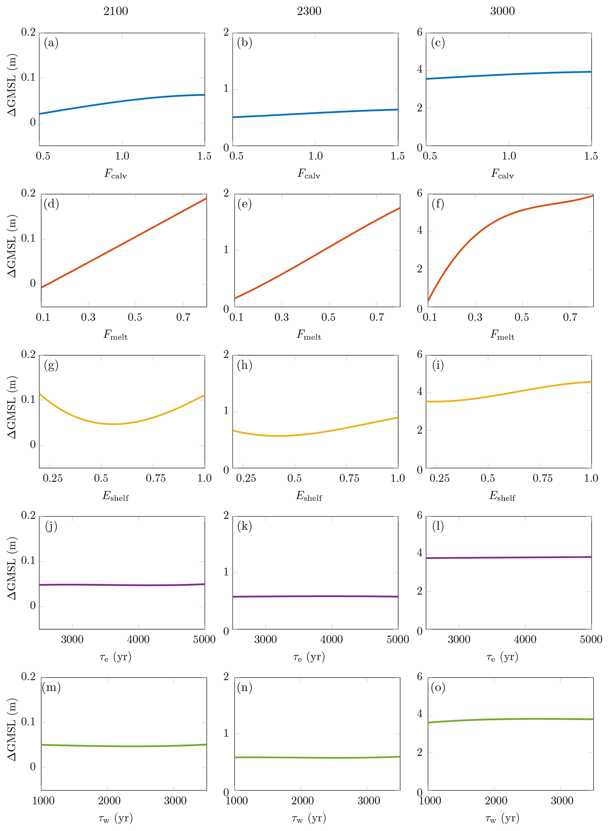
Figure 4a–c show that in RCP 2.6 ΔGMSL increases with an increase in the calving factor non-linearly. The slope is steeper for small values of this parameter, thus suggesting that ΔGMSL is more sensitive to small changes about small values than about higher values. Figure 4d–f indicate that ΔGMSL increases rather linearly with an increase in the melt factor. Figure 4g–i indicate a rather quadratic dependence on the shelf anisotropy factor for short-term and medium-term projections, with small and large values of this factor leading to more significant ice loss than the nominal value. This quadratic dependence can be explained by the influence of E_shelf on two competing processes: a higher value of E_shelf softens the ice, thus leading to faster ice flow in the ice shelves, but a higher value of E_shelf also leads to ice-shelf thinning, thus reducing ice flux at the grounding line. In addition, we find that ΔGMSL depends only little on the bedrock relaxation times (Fig. 4j–o). In fact, lower bedrock relaxation times do tend to stabilise the ice sheet and lower sea-level rise, but this impact is weak compared to the influence of the other parameters. This result may be explained by our orders of magnitude of the bedrock relaxation times being of the order of a few millennia, thus preventing any significant uplift in the next few centuries. Yet, a recent study by Barletta et al. (2018) has suggested a bedrock relaxation timescale of the order of decades to a century in the Amundsen Sea sector, thus making glacial isostatic adjustment significant in the next decades and centuries in this region. To assess the influence of shorter relaxation times, we performed additional numerical experiments, albeit not reported in this paper, with a relaxation time for the whole West Antarctic ice sheet that varies widely from a few decades to a few millennia. For this range of values, we found that bedrock relaxation has a more significant influence on the AIS response, with a contribution to the uncertainty in ΔGMSL that can reach 10 % in RCP 2.6 when τ_w is allowed to vary widely between 50 and 3500 years.

We find in RCP 8.5 similar trends. However, whereas F_calv, F_melt and E_shelf influence ΔGMSL equally in RCP 2.6, the melt factor influences ΔGMSL most significantly in RCP 8.5. Whereas Fig. 5d–e show that ΔGMSL increases rather linearly with an increase in the melt factor, Fig. 5f shows that ΔGMSL rather levels off at a plateau for large values of F_melt for long-term projections in RCP 8.5.

Additionally, Fig. S2 shows the emulators for several pairs of parameters with the other parameters fixed at their nominal values in RCP 2.6 and RCP 8.5. These figures show essentially the same trends as those identified in Figs. 4 and 5, in addition to interaction effects between the parameters. In particular, we find that smaller values of the calving and melt factors lead to mass gain (Fig. S2c), while larger values of the shelf anisotropy and melt factors lead to an important mass loss (Fig. S2d).

3.3 Sea-level rise projections

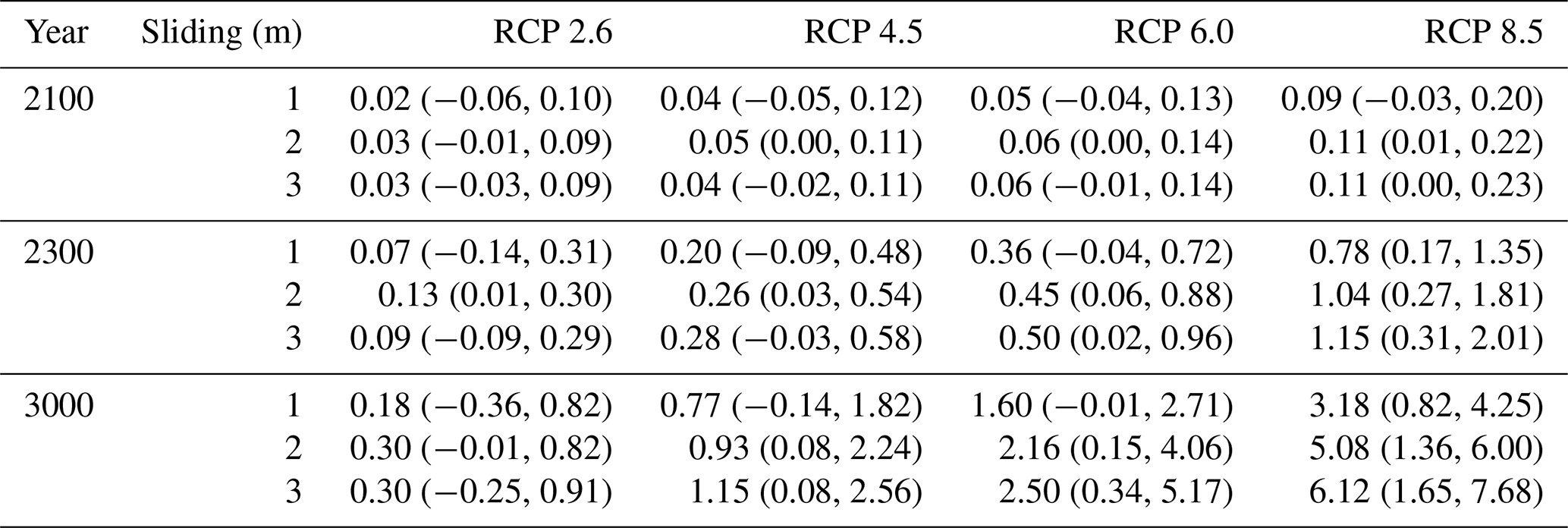
Under parametric uncertainties, we find (Table 3, Fig. 6) in RCP 2.6 a median AIS contribution to sea level that ranges from 0.02 to 0.03 m by 2100, from 0.07 to 0.13 m by 2300 and from 0.18 to 0.30 m by 3000 for the three sliding laws, as compared with the nominal projections of 0.02 m by 2100, 0.07 m by 2300 and 0.20 m by 3000; and we find in RCP 8.5 a median AIS contribution to sea level that ranges from 0.09 to 0.11 m by 2100, from 0.78 to 1.15 m by 2300 and from 3.18 to 6.12 m by 3000, as compared with the nominal projection of 0.05 m by 2100, 0.59 m by 2300 and 3.90 m by 3000. The median AIS sea-level rise projections are higher than the nominal projections, except for certain cases under the viscous sliding law. The nominal projections are not equal to the median projections because the ice-sheet model exhibits non-linearities, as illustrated in Figs. 4 and 5, and the probability density functions for the parameters are not symmetric about their nominal value. As in the nominal projections, we find that in all RCP scenarios and under all sliding laws, the median AIS contribution to sea level is rather small in the first decades and starts to increase around 2100. As in the nominal projections, the median AIS contribution to sea level shows a rather constant growth rate in RCP 2.6, RCP 4.5 and RCP 6.0; contrary to the nominal projection, the median AIS contribution to sea level exhibits initially an acceleration before subsequently exhibiting a deceleration in RCP 8.5 under both non-linear sliding laws (Fig. 6). This behaviour in the median projections in RCP 8.5 is a consequence of the initial rapid collapse of the West Antarctic ice sheet, which contributes 3–3.5 m to sea level, followed by a slower retreat in the East Antarctic ice sheet. By contrast, the nominal projections, which involve a melt factor of 0.3, indicate that the West Antarctic ice sheet does not completely collapse by the year 3000.

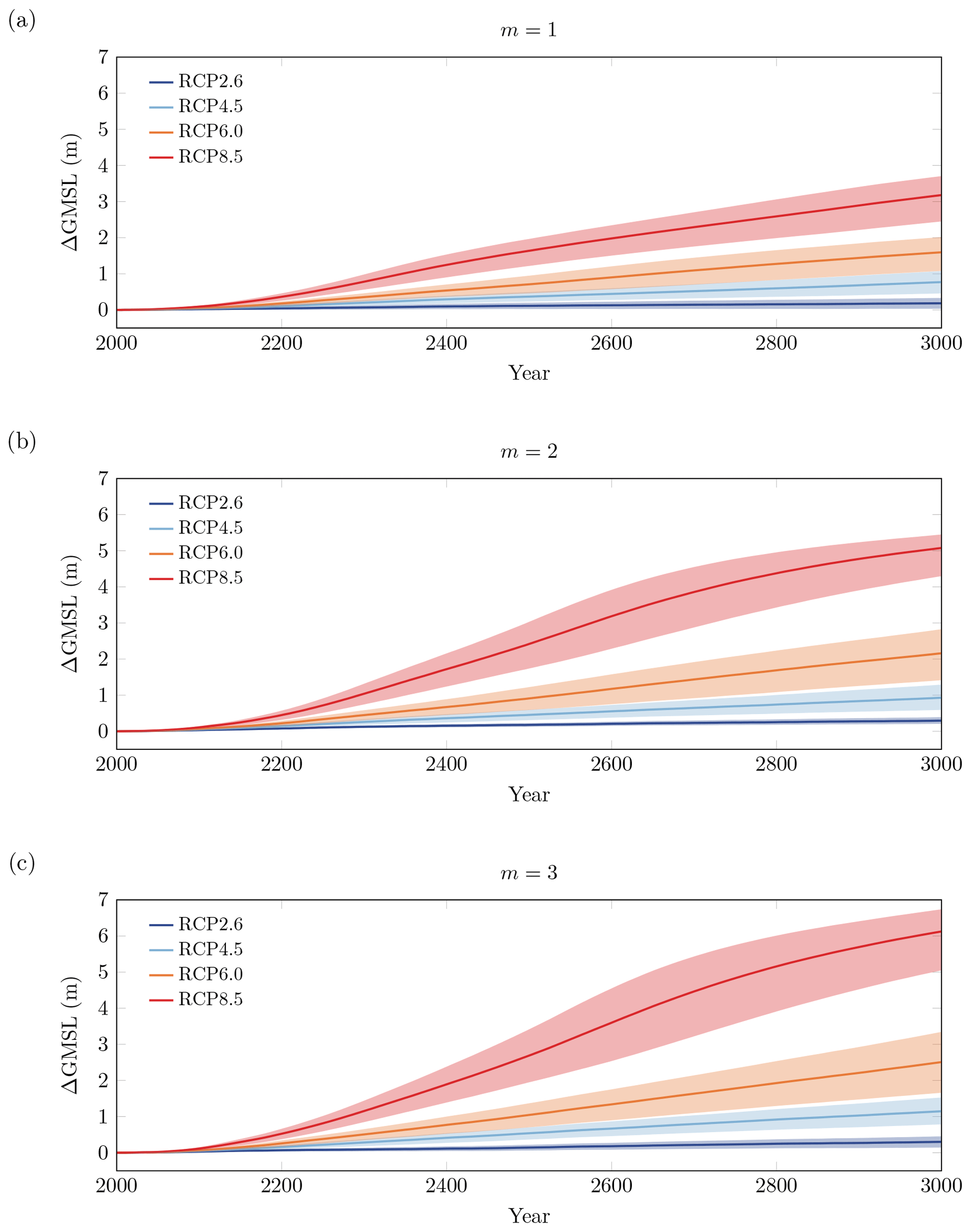
Figure 6AIS contribution to sea level. (a) Viscous sliding law, (b) weakly non-linear sliding law and (c) strongly non-linear sliding law. Solid lines are the median projections and the shaded areas are the 33 %–66 % probability intervals that represent the parametric uncertainty in the model.

Download

In RCP 2.6, we find (Table 3) 5 %–95 % probability intervals for sea-level rise projections that range from −0.06 to 0.10 m by 2100, from −0.14 to 0.31 m by 2300 and from −0.36 to 0.91 m by 3000. In RCP 8.5, these probability intervals range from −0.03 to 0.23 m by 2100, 0.17 to 2.01 m by 2300 and 0.82 to 7.68 m by 3000. The nominal projections are inside the 5 %–95 % probability intervals. We see that the 5 %–95 % probability intervals indicate an increase in sea level, though a decrease cannot be ruled out for the viscous sliding law and cooler atmospheric conditions. Figure 6 highlights that the 33 %–66 % probability intervals become wider under warmer atmospheric conditions and, to a lesser extent, more non-linear sliding conditions. The uncertainty in the projections due to parametric uncertainty is rather significant, with possible overlaps between the 5 %–95 % probability intervals for different RCP scenarios. For instance, Fig. 4i shows that a contribution to sea level of about 0.7 m can be reached by 3000 in RCP 2.6 for the extreme value E_shelf=1, while Fig. 5f shows that this value is reached in RCP 8.5 for very limited sub-shelf melting (F_melt of about 0.12). This suggests that projections with similar contributions to sea level can arise in different RCP scenarios with different combinations of parameter values. Measuring the relative dispersion in ΔGMSL via the coefficients of variation, that is, the ratio between the standard deviation and the mean value, we find a coefficient of variation of 0.74 in RCP 2.6, 0.67 in RCP 4.5, 0.59 in RCP 6.0 and 0.33 in RCP 8.5 by 3000 under the weakly non-linear sliding law. This demonstrates that the relative uncertainty in ΔGSLM projections is higher in cooler RCP scenarios. This results from a much larger increase in the values of ΔGSLM projections compared to the increase in their dispersion when the RCP scenario gets warmer.

Figure 7 shows the probability density functions for the change in GMSL at different timescales. The results display essentially unimodal probability density functions with wider tails for warmer scenarios and longer timescales. In RCP 2.6, the probability density functions resemble Gaussian probability density functions. In RCP 8.5 and at the short and medium timescales, the probability density functions are rather flat, which can be explained by the dependence of ΔGMSL on F_melt being rather linear (Fig. 5d and e). In RCP 8.5 and at the long timescale, the probability density functions exhibit a more localised mode at higher values of ΔGMSL, which can be explained by the collapse of the West Antarctic ice sheet and thus the presence of the plateau for higher values of the melt factor (Fig. 5f).

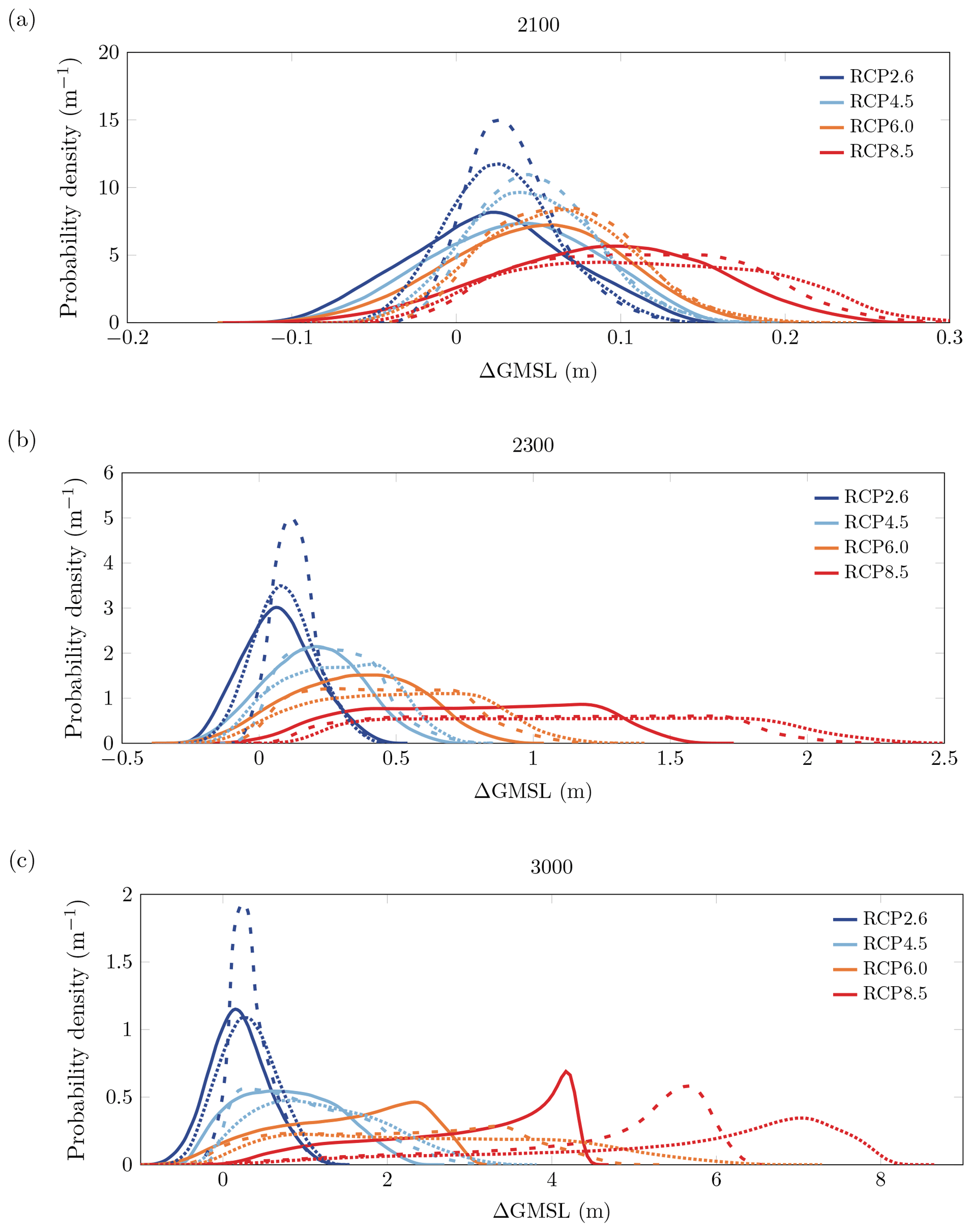
Figure 7Probability density functions for the AIS contribution to sea level at (a) 2100, (b) 2300 and (c) 3000 under the viscous sliding law (solid lines), the weakly non-linear sliding law (dashed lines) and the strongly non-linear sliding law (dotted lines).

Download

Figure 8 gives the probability of exceeding the threshold values of 0.5, 1.0 and 1.5 m as a function of time. We find that the probability of exceeding 0.5 m by 2100 is negligible (probability of less than 1 %) in all RCP scenarios and under all sliding conditions. In RCP 2.6, the AIS contribution to sea level in the next centuries is strongly limited, with a probability of exceeding 0.5 m by 3000 reaching at most 30 %. In RCP 4.5 and RCP 6.0, we found nominal sea-level rise projections well below 1.5 m, while in RCP 8.5 this threshold is exceeded. In the presence of uncertainties, we find that the probability of exceeding 1.5 m of sea-level rise by 3000 can reach about 35 % in RCP 4.5, about 70 % in RCP 6.0 and about 95 % in RCP 8.5. The last result can be seen from Fig. 5, which indicates that ΔGMSL is below 1.5 m only in a small region of the parameter space associated with small values of the melt factor. Furthermore, the shape of the exceedance curves in Fig. 8 provides some insight into the uncertainty in the time when a certain threshold value is exceeded. The time when ΔGMSL exceeds 0.5 m with a probability of 33 % under the weakly non-linear sliding law is 2415 in RCP 4.5, 2270 in RCP 6.0 and 2185 in RCP 8.5, while this value is exceeded with a probability of 66 % at 2790 in RCP 4.5, 2430 in RCP 6.0 and 2245 in RCP 8.5. We find that nominal projections overestimate the time when ΔGMSL exceeds 0.5 m, with the exceedance time being beyond 3000 in RCP 4.5, around 2620 in RCP 6.0 and around 2280 in RCP 8.5.

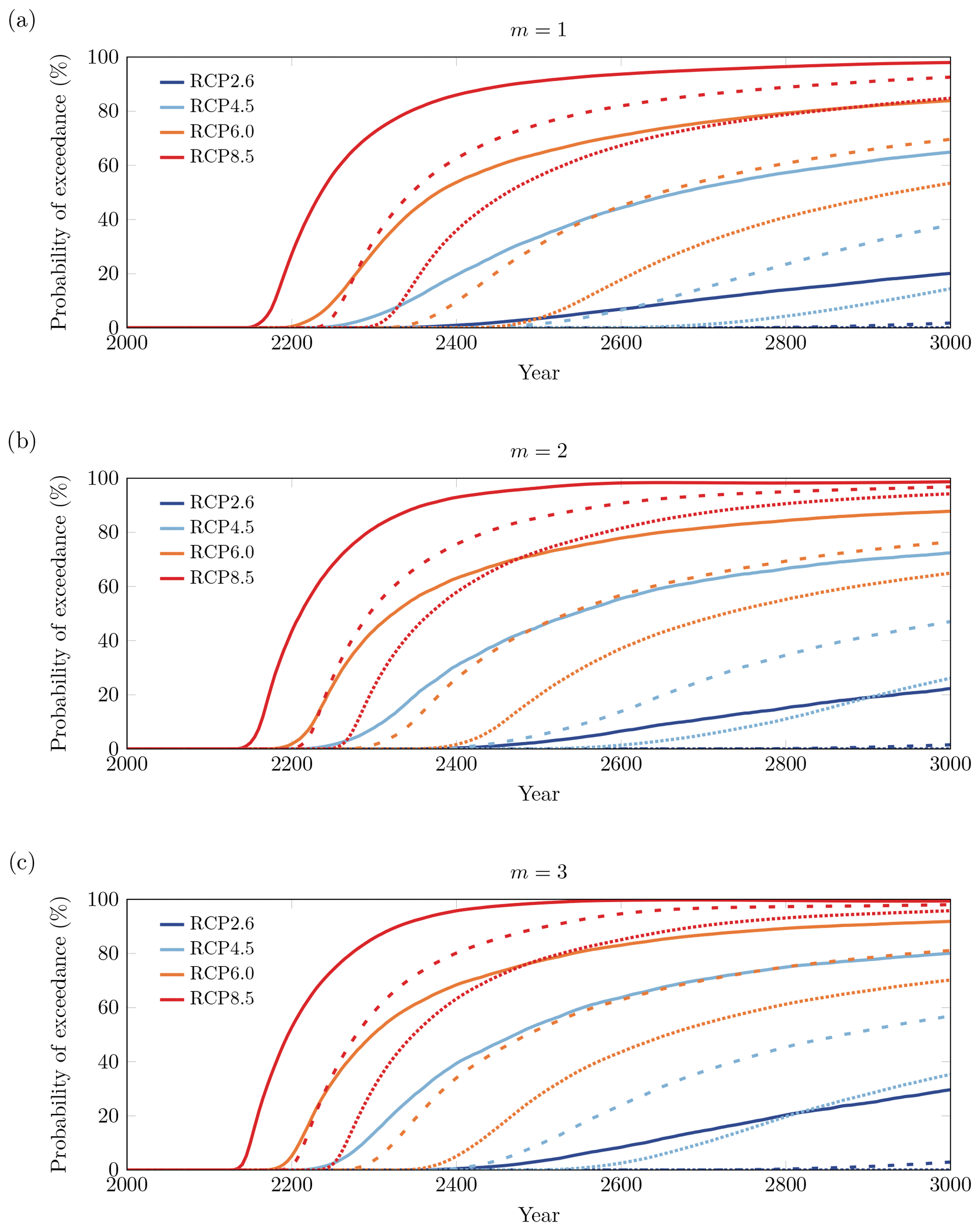
Figure 8Probability of exceeding some characteristic threshold sea-level rise values as a function of time, evaluated from the complementary cumulative distribution functions of the probability density functions for ΔGMSL. Probability of exceedance under (a) the viscous sliding law, (b) the weakly non-linear sliding law and (c) the strongly non-linear sliding law. Solid lines correspond to a threshold value of 0.5 m, dashed lines to a threshold value of 1 m and dotted lines to a threshold value of 1.5 m.

Download

Table 3Probabilistic projections (in metres) of the AIS contribution to sea level on short-term (2100), medium-term (2300) and long-term (3000) timescales in different RCP scenarios and under different sliding conditions with Schoof's grounding-line parameterisation. ΔGMSL projections are the median projections with their 5 %–95 % probability intervals between parentheses.

Download Print Version | Download XLSX

3.4 Stochastic sensitivity analysis

Figure 9 provides the Sobol sensitivity indices for the change in GMSL on short-term, medium-term and long-term timescales in different RCP scenarios and under different sliding laws. We find that in RCP 2.6, the largest contribution to the uncertainty in ΔGMSL stems from the uncertainty in the ice-shelf rheology (Sobol indices ranging from 40 % to 60 %) followed by the uncertainty in the calving rate (Sobol indices ranging from 20 % to 40 %) and sub-shelf melting (Sobol indices ranging from 5 % to 25 %). Indeed, in RCP 2.6, sub-shelf melting plays only a limited role because ocean conditions remain essentially unchanged. Therefore, in RCP 2.6, the dispersion in ΔGMSL is mainly controlled by the ice-shelf rheology, which controls ice flow and buttressing in ice shelves, as well as calving, which reduces the extent of ice shelves and their buttressing.

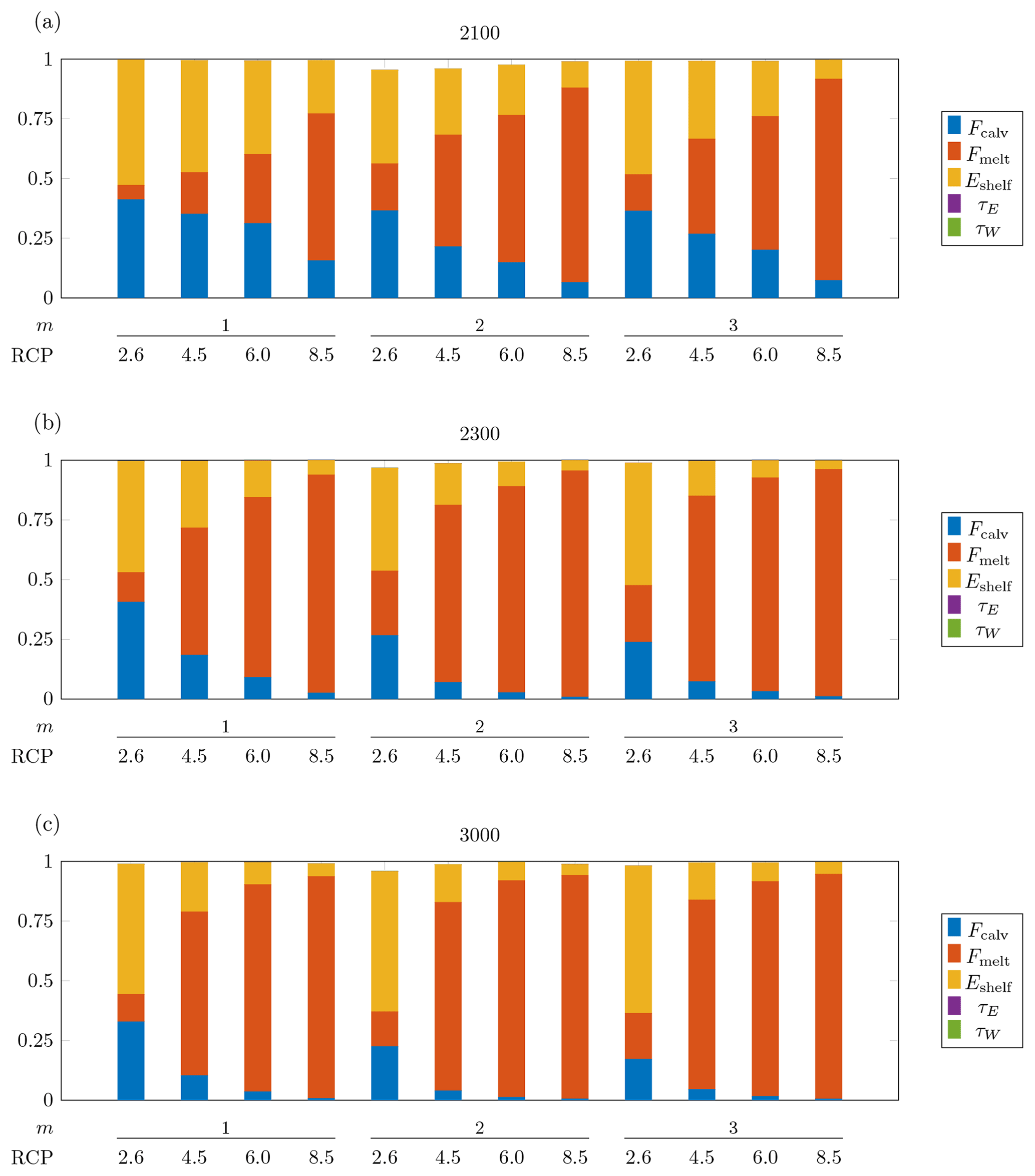
Figure 9Sobol sensitivity indices for the AIS contribution to sea level in different RCP scenarios and for different values of the sliding exponent m in Weertman's sliding law. Sobol indices at (a) 2100, (b) 2300 and (c) 3000. The gap between the height of a bar and the unit value represents the interaction index.

Download

By contrast, in warmer RCP scenarios and for longer timescales, the dominant source of uncertainty becomes the uncertainty in sub-shelf melting, which accounts in RCP 8.5 for more than 90 % of the uncertainty in sea-level rise projections. As shown in Fig. 5, in RCP 8.5 at 3000 ΔGMSL varies by several metres over the range of values of F_melt, while ΔGMSL varies only by a few tens of centimetres over the range of values of the other parameters. Hence, the dominant influence of the uncertainty in the melting factor is also a consequence of the rather wide uncertainty range that we chose for this parameter.

Finally, we find that, in all RCP scenarios and under all sliding laws, the uncertainty in the bedrock relaxation times for West and East Antarctica has a limited impact (Sobol index smaller than 1 %), which is a direct consequence of the very limited dependence of the projections on the bedrock relaxation times. Moreover, the interactions between the parameters have a negligible impact as the sums of the individual Sobol indices account almost entirely for the variances of the projections.

3.5 Projections of grounded-ice retreat

Figure 10 provides insight into the regions of Antarctica that are most at risk of ungrounding in different RCP scenarios and at different timescales under the weakly non-linear sliding law. Figure 10 was obtained as follows. First, we determined the 100 % confidence region for grounded ice, that is, the region of Antarctica where ice is certain to remain grounded, and we coloured it in grey. Thus, there is no risk that the grounding line will retreat to within the grey region. Then, we determined the 95 % confidence region for grounded ice, that is, the region of Antarctica that remains covered everywhere with grounded ice with a probability of more than 95 %, and we coloured the portion of the 95 % confidence region that extends beyond the 100 % confidence region in dark blue. Thus, there is a low risk of (less than) 5% that the grounding line will retreat to within the dark blue region. We continued this procedure for decreasing values of the confidence level and using different colours as indicated in the legend in Fig. 10.

Figure 10Confidence regions for grounded ice under the weakly non-linear sliding law. Confidence regions are shown at (a, d, g, j, m) 2100, (b, e, h, k,n) 2300 and (c, f, i, l,o) 3000. Results under (a–l) the SGL parameterisation and (m–o) the TGL parameterisation.

Download

We find that ice remains grounded in regions above sea level. By contrast, in all RCP scenarios, the risk of ungrounding is highest in marine sectors of West Antarctica with fast-flowing ice streams, especially in Siple Coast, in the Ronne basin, notably Ellsworth Land, and in the Amundsen Sea sector. In warm RCP scenarios and at longer timescales, we also observe a risk of grounding-line retreat in the Wilkes marine basin in East Antarctica, where the grounding line could retreat between 100 km (with a risk of 95 %) and 500 km (with a risk of 5 %) from its present-day position. The risk of retreat in Wilkes basin may partially explain the acceleration in sea-level rise that we observed in Fig. 6 in RCP 8.5. The risk of grounding-line retreat in the Antarctic Peninsula is very limited due to the bedrock topography being above sea level, the marine glaciers being small and a high increase in precipitation in this region.

In RCP 2.6, we observe that the grounding line is quite stable over the next millennium, with the 100 % confidence region for grounded ice being almost unchanged from the present-day grounded ice region (the 100 % confidence region for grounded ice by 3000 only differs from the present-day grounded ice region by a few tens of kilometres). In RCP 4.5, ice remains grounded in most of the West Antarctic ice sheet over the next centuries, but our results also suggest a risk of retreat of the grounding line in some sectors of West Antarctica on longer timescales. In RCP 6.0, we find that the West Antarctic ice sheet belongs by 3000 to the 66 % confidence region for grounded ice, while in RCP 8.5, it belongs by 3000 only to the 5 % confidence region. This suggests a risk of 33 % that a major collapse of the West Antarctic ice sheet might occur in RCP 6.0 by 3000 and a risk of 95 % that a major collapse of the West Antarctic ice sheet might occur in RCP 8.5 by 3000.

As compared with the nominal projections of a limited retreat of the grounding line in West Antarctica in RCP 6.0 by 3000, we find that the impact of the parametric uncertainty is that a complete collapse of the West Antarctic ice sheet may occur with a risk of 33 % in RCP 6.0 by 3000. Moreover, Fig. 3e suggests that a complete disintegration of the West Antarctic ice sheet is underway by 3000 in RCP 8.5, while in Fig. 10l the West Antarctic ice sheet has already collapsed by 3000.

Additionally, we compared the projections under the weakly non-linear sliding law with projections under the other sliding laws, that is, the viscous sliding law (Fig. S7) and the strongly non-linear sliding law (Fig. S8). We find a lower risk of retreat of the grounding line under the viscous sliding law with a slower disintegration of the West Antarctic ice sheet compared to the other sliding laws, especially in the drainage basins of Thwaites and Pine Island glaciers, which belong to the 50 % confidence region for grounded ice by 3000 in RCP 8.5, while they belong to the 5 % confidence region by 3000 in RCP 8.5 for the other sliding laws. The strongly non-linear sliding law seems to favour a faster and deeper retreat of the grounding line, especially in the marine sectors of East Antarctica and the drainage basins of Thwaites and Pine Island glaciers. However, Figs. 10i and S8i suggest that ungrounding may be less significant in Siple Coast under the strongly non-linear sliding law than the weakly non-linear sliding law. Actually, MISI may occur when driving stresses overcome resistive stresses (Waibel et al., 2018). Driving stresses are primarily determined by the surface slopes, while resistive stresses depend on the basal sliding coefficient and the ice velocity through the sliding exponent. Driving stresses at the grounding line are higher in the Amundsen Sea sector than in Siple Coast due to steeper surface slopes, leading to a greater sensitivity of the grounding line in the former region to non-linearity and a more plastic response.

3.6 Influence of the parameter probability density function

So far, we have represented the uncertain parameters F_calv, F_melt, E_shelf, τ_e and τ_w by a uniform distribution on a fixed support. For instance, the uncertain parameter F_calv is represented by a uniform distribution with support $[F_{\mathrm{calv},\min },F_{\mathrm{calv},\max }]$, where F_calv,min and F_calv,max are the minimum and maximum values in Table 1. We now address the influence of the probabilistic characterisation of the parametric uncertainty on our probabilistic projections by controlling the size of these supports. Hence, we represent the uncertain parameters F_calv, F_melt, E_shelf, τ_e and τ_w by a family of uniform probability density functions indexed by a unique scaling factor $\mathit{\alpha }\in [\mathrm{0},\mathrm{1}]$ that controls the supports of the uniform probability density functions. For instance, the uncertain parameter F_calv is represented for a given value of α by a uniform distribution with support $[F_{\mathrm{calv},\mathrm{nom}}+\mathit{\alpha }(F_{\mathrm{calv},\min }-F_{\mathrm{calv},\mathrm{nom}}),F_{\mathrm{calv},\mathrm{nom}}+\mathit{\alpha }(F_{\mathrm{calv},\max }-F_{\mathrm{calv},\mathrm{nom}}\left)\right]$, where F_calv,nom, F_calv,min and F_calv,max are the nominal, minimum and maximum values in Table 1. For the other parameters, the supports are defined similarly. The value α=0 represents the ice-sheet model without parametric uncertainty, that is, the ice-sheet model for the nominal values of the parameters, and the value α=1 represents the full uncertainty ranges considered so far. We propagated the uncertainty from the parameters to the sea-level rise projections for different values of the scaling factor, reusing the emulator that we had built for α=1 over the whole parameter space. Hence, the projections to follow for α=0 based on this emulator are not exactly equal to the nominal projections determined directly from the ice-sheet model.

For the long-term projections, Fig. 11a–d show the median and the 33 %–66 % and 5 %–95 % probability intervals as a function of the scaling factor in the different RCP scenarios under the weakly non-linear sliding law and Fig. 11e–h show the probability density functions for the values $\mathit{\alpha }=\mathrm{0.2},\mathrm{0.6}$ and 1.0. We find that the median projections increase with an increase in the scaling factor and range in RCP 2.6 from 0.16 to 0.30 m, in RCP 4.5 from 0.37 to 0.93 m, in RCP 6.0 from 1.11 to 2.16 m and in RCP 8.5 from 3.80 to 5.08 m. In addition, the width of the probability intervals increases with increasing uncertainty in the parameters. While the width of the 33 %–66 % probability interval increases rather linearly with the scaling factor and is rather symmetric about the median, the width of the 5 %–95 % probability interval increases more non-linearly with an increase in the scaling factor, as illustrated in Fig. 11a in RCP 2.6 and Fig. 11d in RCP 8.5. The probability density functions attribute higher weight to larger values of ΔGMSL under increased parametric uncertainty, with increased weight given to larger values of in particular E_shelf in RCP 2.6 (Fig. 4i) and F_melt in RCP 8.5 (Fig. 5f). Figure 11a–d show that the sensitivity of the amount of uncertainty in the projections (probability intervals) to the amount of uncertainty in the parameters (scaling factor) is higher for warmer scenarios, with an upper bound between RCP 6.0 and RCP 8.5 as a consequence of the collapse of the West Antarctic ice sheet.

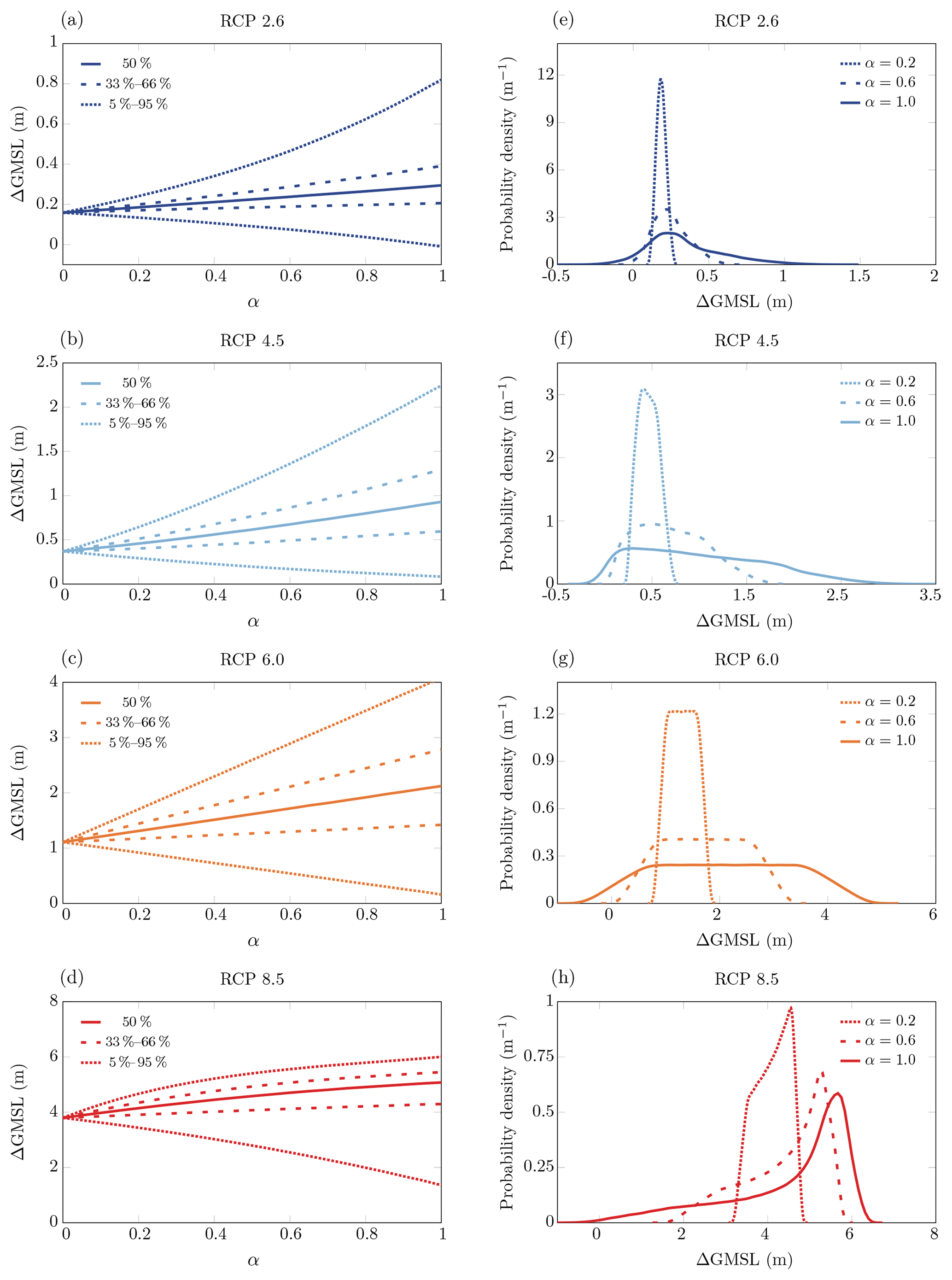
Figure 11Robustness of probabilistic projections with respect to the scaling factor α. Median projections and their 33 %–66 % and 5 %–95 % probability intervals by 3000 under for the weakly non-linear sliding law in (a) RCP 2.6, (b) RCP 4.5, (c) RCP 6.0 and (d) RCP 8.5. Probability density functions for α=0.2 (dotted lines), α=0.6 (dashed lines) and α=1 (solid lines) in (e) RCP 2.6, (f) RCP 4.5, (g) RCP 6.0 and (h) RCP 8.5.

Download

3.7 Projections under a more plastic sliding law

We ran the same ensemble of simulations under a more plastic sliding law (m=5). Table 4 and Fig. 12 give for the AIS contribution to sea level the median and the 33 %–66 % and 5 %–95 % probability intervals. As compared with less plastic sliding laws ($m=\mathrm{1},\mathrm{2},\mathrm{3}$), we find an increase in sea-level rise projections on short-term and medium-term timescales, thus suggesting a more significant and faster response to perturbations under more plastic sliding conditions. On a long-term timescale, the ice-sheet mass loss can be less important under m=5 than m=3, as observed in the median projections by 3000 in RCP 4.5 and RCP 8.5.

Figure 12Same as Fig. 6 but under Weertman's sliding law with exponent m=5.

Download

We find that overall the AIS contribution to sea level is an increasing function of the sliding exponent, with the differences between successive exponents getting smaller as m increases, as already pointed out by Gillet-Chaulet et al. (2016); for instance, we observe a greater difference in the projections between m=1 and m=2 than between m=3 and m=5. On longer timescales, tipping points and non-linearities associated with MISI may trigger a slightly different response of the ice sheet depending on the initial conditions, which could explain the smaller ice loss in our results under m=5 than m=3.

Table 4Same as Table 3 but with sliding exponent m=5. ΔGMSL projections are the median projections with their 5 %–95 % probability intervals between parentheses.

Download Print Version | Download XLSX

3.8 TGL parameterisation

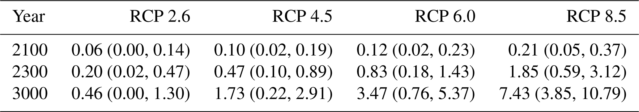
We ran the same ensemble of simulations under the weakly non-linear sliding law using, this time, the TGL parameterisation instead of the SGL parameterisation. Under the TGL parameterisation, Table 5 and Fig. 13 give for the AIS contribution to sea level the median and the 33 %–66 % and 5 %–95 % probability intervals. We find an overall increase in sea-level rise projections compared to our results under the SGL parameterisation. This result was expected as the TGL parameterisation has been shown to increase grounding-line sensitivity to environmental changes (Tsai et al., 2015; Pattyn, 2017). The probability of exceeding 0.5 m by 2100 is still negligible (probability of less than 1 %) in all RCP scenarios. However, the probability of exceeding 0.5 and 1 m by 3000 in RCP 2.6 can reach more than 40 % and 10 %, respectively. For other scenarios, the retreat of the Antarctic ice sheet is much more pronounced and faster than under the SGL parameterisation, and the probability of exceeding 1.5 m of sea-level rise by 3000 can reach more than 50 % in RCP 4.5, 80 % in RCP 6.0 and 99 % in RCP 8.5.

Figure 13Same as Fig. 6 but under the TGL parameterisation and the weakly non-linear sliding law.

Download

Figure 10m–o show the confidence regions for grounded ice under the TGL parameterisation in RCP 8.5. As also pointed out by Pattyn (2017), the TGL parameterisation leads to a faster and more significant grounding-line retreat in the marine sectors and an additional mass loss from East Antarctica, especially in the Aurora basin.

Table 5Same as Table 3 but with the TGL parameterisation. ΔGMSL projections are the median projections with their 5 %–95 % probability intervals between parentheses.

Download Print Version | Download XLSX

4.1 Comparison of the sea-level rise projections with previous work

Regarding the short-term AIS contribution to sea level, we projected in the RCP 2.6 scenario a median of 0.02–0.03 m under the SGL parameterisation and 5 %–95 % probability intervals from −0.06 to 0.10 m. These projections are similar to other estimates based on other mechanisms. Golledge et al. (2015) reported an AIS contribution to sea level between −0.01 and 0.10 m with the lower and higher bounds corresponding to the absence and presence of sub-grid interpolation of basal melting at the grounding line. DeConto and Pollard (2016) reported an AIS contribution to sea level between −0.11 and 0.15 m based on a model calibration with a range of Pliocene sea-level targets between 5 and 15 m higher than today. In the same scenario, we found an increased AIS response under the TGL parameterisation with a median AIS contribution to sea level of 0.06 m and a 5 %–95 % probability interval between 0.00 and 0.14 m by 2100. These higher projections are similar to the higher projections (0–0.22 m) reported by DeConto and Pollard (2016) for a higher range of Pliocene sea-level targets between 10 and 20 m. In all RCP scenarios, under all sliding laws and under both grounding-line parameterisations, our results suggested that the AIS contribution to sea level does not exceed 0.5 m by 2100, with a probability of at least 99 %. These results are in agreement with Ritz et al. (2015), who determined an AIS contribution to sea level that lies between 0.05 and 0.30 m, and Golledge et al. (2015), who found an AIS contribution to sea level that reaches at most 0.38 m in RCP 8.5 with sub-grid interpolation of basal melting at the grounding line. Yet, projections by DeConto and Pollard (2016) and Schlegel et al. (2018), who applied the more sensitive Budd-type friction law (Brondex et al., 2017), can exceed 0.5 and even 1 m, but these higher projections are under extreme and maybe unrealistic warming conditions.

Regarding the long-term AIS contribution to sea level, our projections under the SGL parameterisation are similar to other estimates by Golledge et al. (2015). In particular, both studies suggest that the AIS contribution to sea level by 3000 in RCP 2.6 is limited to less than 1 m with a probability estimated to be at least 95 % in our study, while an AIS contribution to sea level above 1.5 m by 3000 may arise in all other RCP scenarios. Yet, our long-term projections are generally below projections by DeConto and Pollard (2016) with hydrofracturing and ice-cliff failure mechanisms especially under warmer RCP scenarios, but the discrepancies between the projections of both models are reduced under the TGL parameterisation. In RCP 2.6, our projections by 2500 under the TGL parameterisation range from 0.04 to 0.73 m, which is similar to projections by DeConto and Pollard (2016), which range respectively from −0.23 to 0.61 m and 0.02 to 0.48 m for the lower and higher ranges of Pliocene of sea-level targets.

4.2 Comparison of the impact of parametric uncertainty with previous work

Similarly to Golledge et al. (2015, 2017), our study emphasised the pivotal role played by the emission scenario and sub-shelf melting as critical drivers of the future changes in the AIS mass balance on medium-term and long-term timescales through ice-shelf thinning and subsequent reduced buttressing. As in Ritz et al. (2015), we found that the AIS contribution to sea level is an increasing function of the sliding exponent, thus meaning that more plastic sliding conditions speed up the ice flow and consequently ice loss. Following Pattyn (2017), we highlighted the greater sensitivity of the grounding-line migration under the TGL parameterisation, thus stressing the key role played by physical processes in the vicinity of the grounding line.

4.3 Comparison of projections of grounded-ice retreat with previous work

Consistent with our results, Golledge et al. (2015), with a 10 km resolution model, projected that grounding-line retreat is most significant in the Siple Coast region. However, Ritz et al. (2015), based on the probability of MISI onset, as well as Cornford et al. (2015), with a sub-kilometre resolution around the grounding line, projected that grounding-line retreat is most significant in the Amundsen Sea sector. Schlegel et al. (2018) found that grounding-line retreat is most significant in the Amundsen Sea sector under generalised ocean warming experiments for the Antarctic ice sheet, but, after calibrating sub-shelf melt rates with bounds that vary region by region and are assigned values deduced from the literature and model sensitivity studies, they found that the western Ronne basin has the greater sensitivity. These discrepancies between our findings and those of Cornford et al. (2015), Ritz et al. (2015) and Schlegel et al. (2018) may be explained by our ocean model which may overestimate sub-shelf melting underneath the Ross ice shelf and underestimate ocean circulation in the Amundsen Sea and by our initialisation method which may underestimate the basal sliding coefficients for Thwaites and Pine Island glaciers. Moreover, the lower sensitivity of the Amundsen Sea sector may arise in our simulations from shortcomings in the buttressing parameterisation, our low resolution not capturing properly the bedrock topography, the small pinning points and the flow dynamics in the narrower sectors of the ice sheet and our representation of calving, which may increase the instability threshold; see, for instance, Arthern and Williams (2017) and Waibel et al. (2018) for more thorough discussions about the instability threshold in the Amundsen Sea sector.

4.4 Projections of ice loss and grounding-line retreat under parametric uncertainty

The significance of the contribution of the Antarctic ice sheet to sea level under climate change is primarily controlled by the sensitivity, the response time and the vulnerability of its marine drainage basins, with the West Antarctic ice sheet more sensitive and vulnerable than the East Antarctic ice sheet. The instability of marine drainage basins and their ability to trigger accelerated ice loss and significant grounding-line retreat is determined by bedrock topography and ice-shelf buttressing which depends on the importance of ice-shelf thinning. Our nominal projections showed that the AIS contribution to sea level by 3000 is rather limited (less than 1 m) in RCP 2.6, RCP 4.5 and RCP 6.0, while an accelerated ice loss that leads to a contribution of several metres is triggered in RCP 8.5 (Fig. 3a). In addition, the nominal retreat of the grounding line by 3000 is rather limited in RCP 2.6, RCP 4.5 and RCP 6.0 (Fig. 3b–d), while a significant retreat of the grounding line is triggered in the Siple Coast, Ronne–Filchner and Amundsen Sea sectors in RCP 8.5 (Fig. 3e).

Our probabilistic results provide insight into the impact of parametric uncertainty on these projections. In RCP 2.6, the projections hold irrespective of parametric uncertainty: the AIS contribution to sea level by 3000 has a 95 % quantile of up to 0.91 m (Table 3) and there is a limited risk that the grounding line will retreat beyond our nominal projections (Figs. 3b and 10c). In RCP 4.5 and RCP 6.0, the projections are more sensitive to parametric uncertainty than in RCP 2.6: the AIS contribution to sea level by 3000 has a 95 % quantile of up to 2.56 m in RCP 4.5 and up to 5.17 m in RCP 6.0 (Table 3), and both scenarios entail a risk of triggering a more significant retreat of the grounding line beyond our nominal projections (Fig. 3c–d). This risk is present especially in the Amundsen Sea sector, and it is less significant in RCP 4.5 than in RCP 6.0, in which a complete disintegration of the West Antarctic ice sheet may be triggered (Fig. 10f and i). Finally, in RCP 8.5, our probabilistic results suggest an accelerated ice loss and a significant retreat of the grounding line in West Antarctica, as in our nominal projections: the AIS contribution to sea level by 3000 has an uncertainty range with a 5 % quantile above 0.82 m and a 95 % quantile of up to 7.68 m (Table 3), and there is a high risk of triggering a complete disintegration of the West Antarctic ice sheet (Fig. 10l).

In conclusion, the projections hold irrespective of parametric uncertainty in the strongly mitigated RCP 2.6 scenario: accommodating parametric uncertainty in the ice-sheet model leads to projections in agreement with the nominal projections of limited ice loss and limited grounding-line retreat in RCP 2.6. However, the projections are more sensitive to parametric uncertainty for intermediate scenarios such as RCP 4.5 and RCP 6.0: accommodating parametric uncertainty in the ice-sheet model leads to projections in disagreement with the nominal projections and indicates instead some risk of triggering accelerated ice loss and significant grounding-line retreat for intermediate scenarios such as RCP 4.5 and RCP 6.0. Finally, the warm RCP 8.5 scenario triggers the collapse of the West Antarctic ice sheet, almost irrespective of parametric uncertainty.

4.5 Structural uncertainty and limitations

A first limitation of our study is associated with the modelling hypotheses inherent to our ice-sheet model. The f.ETISh model is an ice-sheet model that focuses on essential marine ice-sheet mechanisms, similarly to the ice-sheet model by Pollard and DeConto (2012a). Certain physical processes, especially small-scale processes, may be represented imperfectly, especially with the 20 km resolution adopted for our simulations. This may reduce the ability to simulate important ice streams such as Pine Island and Thwaites glaciers (only represented by a few grid points), whose stability is controlled by local bedrock features (Waibel et al., 2018). Hence, grounding-line migration and thresholds for instabilities may not be captured properly even with a parameterisation of the grounding-line flux, especially in low-forcing scenarios and short-term projections. As discussed in Sect. 2.1, the flux condition at the grounding line is also questionable for buttressed ice shelves (Pattyn et al., 2013; Reese et al., 2018a) found around Antarctica and short transients (Drouet et al., 2013; Pattyn et al., 2013; Pattyn and Durand, 2013). Yet, we think that using a 20 km resolution and a flux condition at the grounding-line remains an acceptable assumption in large-scale and long-term ice-sheet simulations and large-ensemble simulations. We expect discrepancies between our results and results at a higher spatial resolution or with a higher level of complexity to be limited when compared to the uncertainty in the results due to the uncertainty in the model parameters and forcing. Besides, sub-shelf melting may not be captured properly despite the use of the PICO ocean-model coupler, especially in the Amundsen Sea sector and underneath the Ross ice shelf (Timmermann et al., 2012; Depoorter et al., 2013; Rignot et al., 2013; Moholdt et al., 2014). A second limitation comes from the hypotheses relevant to our characterisation of uncertainties. We adopted rather large uncertainty ranges for the parameters. As discussed in Sect. 3.6, projections can be strongly affected by extreme conditions. Moreover, we chose the bounds of the uncertainty ranges quite heuristically. A third limitation comes from the fairly simple way in which certain sources of uncertainty were introduced. We assumed a direct influence of the atmospheric forcing on sub-shelf melting through the ocean melt factor. However, as discussed in Sect. 2.2.5, atmospheric forcing affects the Circumpolar Deep Water circulation in ice-shelf cavities and subsequently modifies sub-shelf melting (Pritchard et al., 2012). Still, the fate of the Southern Ocean and the evolution of sub-shelf melting under global climate change remains unclear (Hellmer et al., 2012; Dinniman et al., 2012; Timmermann and Hellmer, 2013; Hellmer et al., 2017). Given the importance of sub-shelf melting in driving the future response of the Antarctic ice sheet, there is a clear need to better constrain future sub-shelf melt and incorporate it properly into ice-sheet models. We also introduced uncertainty in calving with a simple multiplier factor that does not take into account the stress regime in the ice shelves. A fourth limitation concerns the correction for the initial drift that adds a bias to the projections. We adopted this correction to make our results insensitive to model initialisation, but our corrected results are likely to underestimate the AIS response on a short-term timescale, as our approach does not take into account any current transient changes in the Antarctic ice sheet. Another limitation is related to the construction of our emulator. To avoid overfitting the training data, we tuned the emulator to reproduce the overall trend in the parameters-to-projection relationship, but not local variations in the parameter space that may stem from numerical noise and errors.